MATLAB is a command-line (mostly) numerical (mostly) computation program. It is designed for matrix math, but deals very well with sets of data, since a column of numbers is essentially a vector, which mathematically is just a 1D matrix.
Getting data into MATLAB
MATLAB interprets a set of data as a list of numbers. You can manually enter data by typing a name for the data, “=”, and then the data itself as a list inside square brackets.
mydata = [1 3 6 10.0]
If you already have your numbers on the clipboard (because you just copied them from somewhere), you can simply paste (for instance, using Ctrl-V) instead of typing them, but remember to finish off with the closing square bracket.
mydata = [ Ctrl-V ]
You can sometimes paste in multiple columns of data, but MATLAB is picky about this. For instance, you will be rejected if you try to paste columns of different lengths.
You can separate items by commas if you like; if you separate them by semicolons you will create a column rather than a row – this is unlikely to affect anything. Note that the MATLAB terminology for a 1D set of data (a column or row in Excel) is a column or row vector. To manually edit your data, double-click on its name in the Workspace viewer: it will open in a spreadsheet-like display where you can change, delete or add entries. Append a semicolon to the end of a command to prevent MATLAB from printing the result; the result it still calculated normally, it’s just not displayed onscreen.
You can reference specific portions of a vector using parentheses ():
initial_x = x(1)
first_ten_values = mydata(1:10)
Note that MATLAB indexes starting from 1 (not 0); the last entry can be referenced as end:
last_x = x(end);
Performing calculations with data
MATLAB calculations are done from the command line. Normal functions work as expected, e.g.
newdata = olddata*2+17;
data_in_m = data_in_mm/1000;
ells=100*cos(theta);
However, when you perform calculations with two vectors, (1) they must be exactly the same size, and (2) you must preface some operands (usually multiplication (*), division (/), and exponentiation (^)) with a period. (This occurs because MATLAB interprets * as matrix multiplication, which is a different beast. As long as you don’t want matrix multiplication (and you probably don’t) there is no harm in using .* instead of * even when it’s not necessary).
v = dx ./ dt;
If you just type a calculation without using the = sign to assign it to a new variable, the result is stored in the variable ans. You probably don’t want to do this because ans will get written over the next time you do something similar.
Some functions change the size of the data. For instance, diff(x) constructs the difference vector [x[2]-x[1], x[3]-x[2], … x[end]-x[end-1]], which is one shorter than x was. In the example below, x is one entry longer than dx:
dx = diff(x)
This behavior would be pretty obvious if you coded in Excel, but may surprise you in MATLAB.
Graphing
The basic graphing command in MATLAB is plot(). This will pop up a new window with a basic plot in it; the window contains a menu bar with commonly used graphing commands (such as changing line color, adding axis labels, changing axis limits, etc.) though those may also be changed using the command line.
The simplest plotting command is
plot(xdata,ydata)
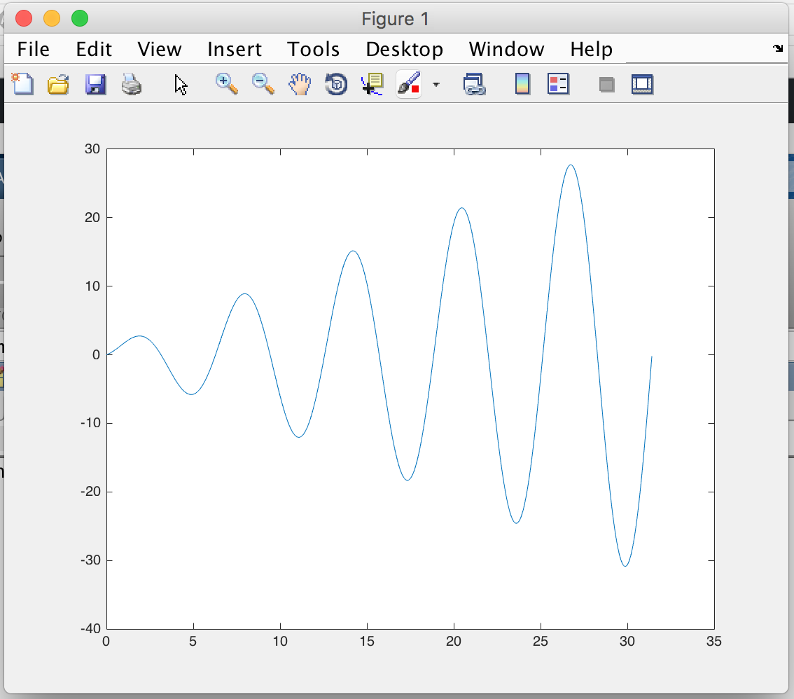 The resulting plot window is pretty basic, but you can adjust it using the commands in the menubar at the top of the figure window. The most useful ones are
- Insert > X Label (and similar commands) to add axis labels, legend, and annotations
- Edit > Axes Properties to change the axis limits, tick marks, etc.
- The line properties editor (double-click the data plot) to change the color, symbol, thickness, etc. of the plotted data line.
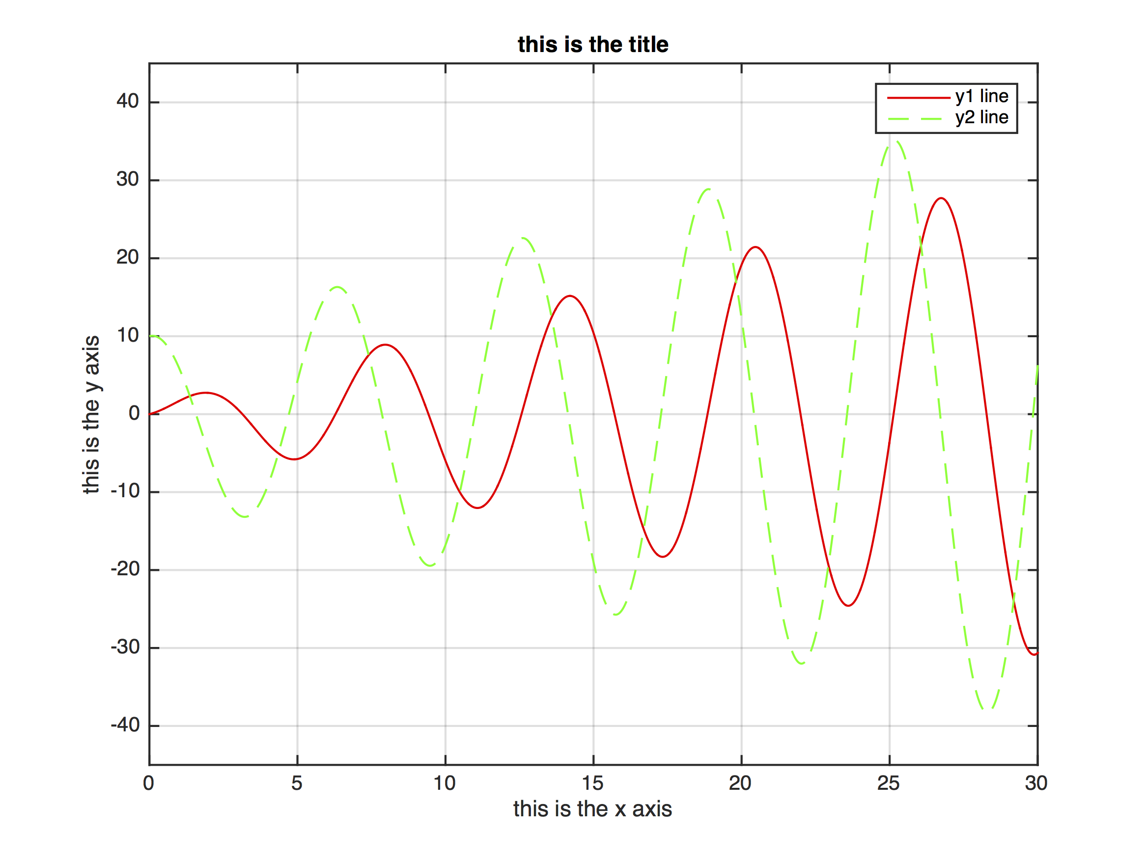
Alternatively, you can tweak the exact look of the graph using the command line for instance:
x = 0:0.01:10*pi; % generate numbers from 0 to 10π with a spacing of 0.01
y1 = sin(x).*(1+x); % compute y from x
y2 = cos(x).*(10+x); % compute another y from x
plot(x,y1,'r-',x,y2,'g--'); % plot each y vs x with lines 'r-' (solid red) and 'b:' (dashed green)
axis([0 30 -45 45]); % change axis limits to [xmin xmax ymin ymax]
xlabel 'this is the x axis'
ylabel 'this is the y axis'
title 'this is the title'
grid on % turn on the x and y gridlines
legend('y1 line','y2 line') % add legend to graph
 Getting graphics out of MATLAB
You can usually cut/paste a figure directly from the figure’s window into Word or Powerpoint or similar applications. If necessary, use File > Save As to create a file with a specific graphic format that you like; generally, vector graphics formats (SVG, PNG, EPS, PDF) perform better than bitmapped ones.
Histogramming in MATLAB
MATLAB has an elegant histogramming command that calculates selects bins, calculates frequencies and creates a bar plot in a figure window. This can all be done automatically, or you can tweak the behavior by specifying parameters to get a prettier plot.
In order of increasing user control, you can use
histogram(mydata) % completely automatic bins
histogram(mydata,10) % 10 automatic bins
histogram(mydata,[0 2 4 6]) % 3 bins, with the ranges (edges) {0-2,2-4, and 4-6}
For instance, the code below generates and then histograms some data:
grades = 50+10*randn(1000,1); % generate random numbers
histogram(grades,[0 10 20 30 40 50 60 70 80 90 100]) % calculate and display histogram with bin edges as given
axis([0 100 0 500]) % set pretty axis limits
xlabel 'grade'
ylabel 'number of occurrences'
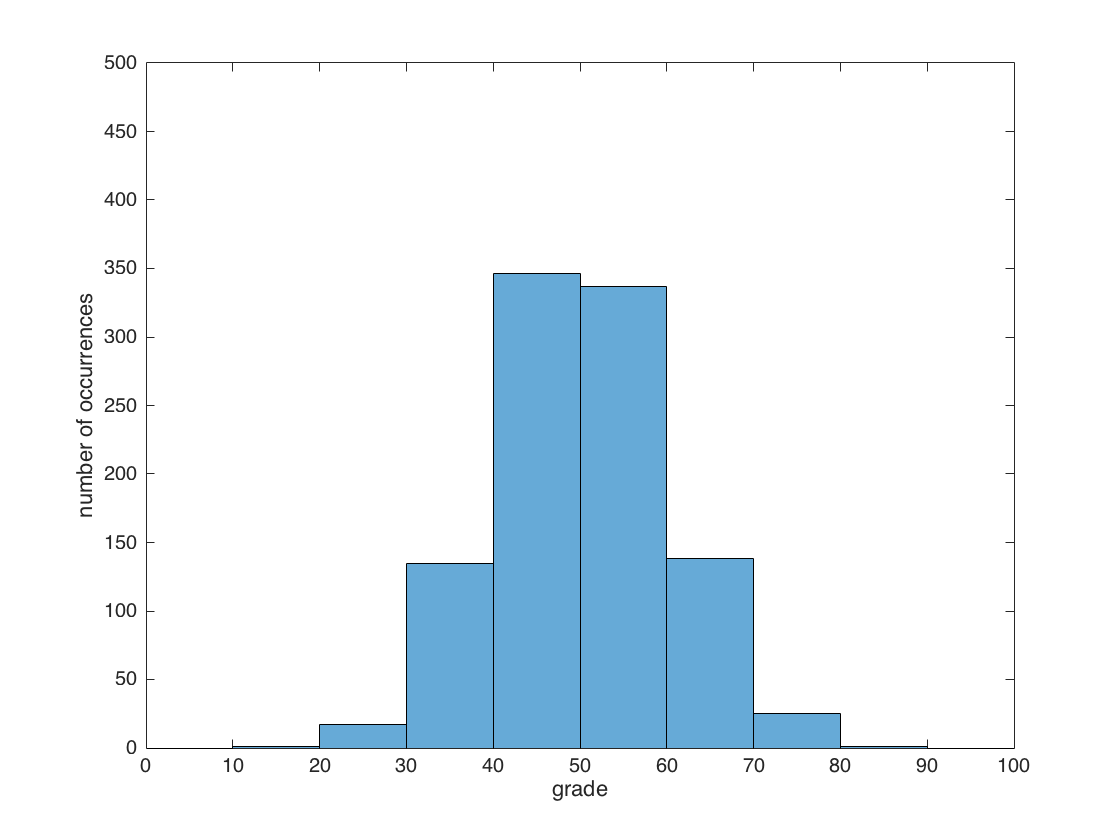
- It would have been easier to type the bin edges vector as 0:10:100, which is “a vector containing numbers that start at 0, incrementing by 10 until they reach 100”
- The axis adjustment and labeling can be done by selecting commands from the figure window if you prefer to point and click.
- I usually start by letting MATLAB generate the histogram completely automatically – i.e. I just type histogram(mydata). Based on that, I decide how to adjust the bins to make the graph more readable, and then rehistogram it with my own bins.