Motivation
In this final lab, we will be exploring the interaction of light with matter. Using spectroscopy (also called spectral analysis, spectrometry, or spectrophotometry), we will examine emission and absorption of light by various substances. Spectrometers (also called spectrophotometers) are measurement tools designed to distinguish different colors of light. The spectrometers we will use in this lab detect the intensity of the light (the power-per-area associated with the light) as a function of the wavelength of the light. These spectrometers have a sensitivity range from 350 nm to 1000 nm, with a spectral resolution of 2 nm. In contrast, the human eye has a sensitivity range from approximately 400 nm (violet) to 700 nm (red), with a spectral resolution ranging from 1 nm (in the green to yellow range) to 10 nm (in the violet and red ranges). You may have been exposed to spectroscopy data through your previous chemistry and biology courses. To thoroughly understand data, one must know where it came from, its limitations, and its interpretations and potential meanings. With this lab we hope to deepen your comprehension of the function of spectrometers and thereby enrich your understanding of the data they produce. This will lay a firm foundation for your use of spectroscopy in your broader scientific career.
Matter has rich internal activity. Since matter is bound together in stable situations by forces, it has lots of natural ways to oscillate and resonate. The methyl groups on organic molecules can spin around. Similarly, long molecular chains can vibrate back-and-forth like a spring. Within each atom, electrons are constantly shifting towards and away from the nucleus. Each of these processes has a particular wavelength (color) of light associated with it: a specifically-sized photon energy packet is emitted or absorbed. Since light can only be absorbed or emitted in these packets, the way different colors of light interact with matter tells us about the energy spacing between the allowed excitation states of atoms and molecules. Doing a spectral analysis of light emitted or absorbed by something can give us a lot of information about it. Stokes (famous for his study of viscosity) was the first to show that hemoglobin was the molecule responsible for carrying oxygen in the blood—he did this using spectral analysis! On an entirely different physical scale, it’s spectral analysis that permits us to figure out the composition of stars.
Your lab will consist of three parts: I) exploring the quantized atom; II) exploring emission and absorption; and III) analyzing the emission spectrum of chlorophyll. The lab report you turn in at the end of this investigation should discuss answers to questions posed in the sections below as well as any insights you gain from your explorations and investigations, along with the data supporting those insights.
A Short Introduction to Light and Photons
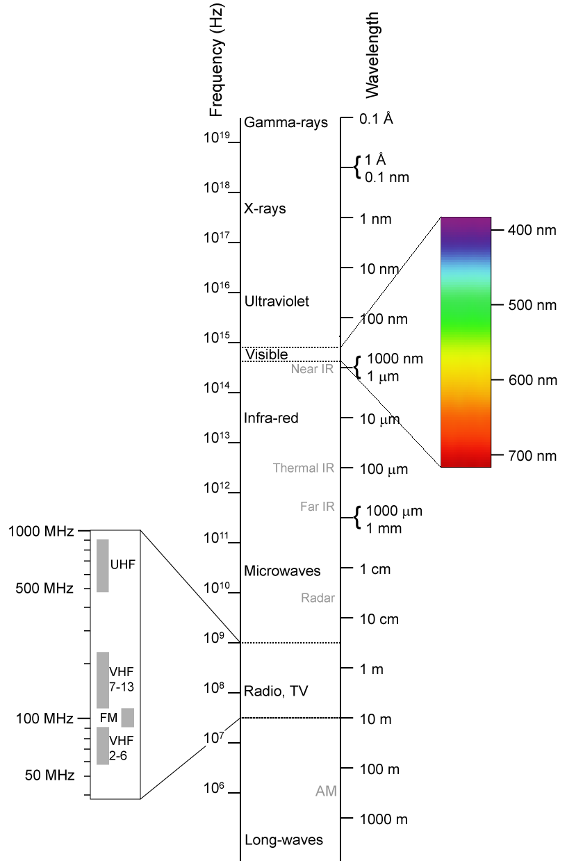 The range of all possible light waves is referred to as the Electromagnetic (EM) Spectrum Of this range, the visible portion (sensed by the human eye, roughly 400 nm – 700 nm) is only a very small section.
- All light waves move at a speed of c = 3.0 × 10⁸ m/s in a vacuum. In a medium other than vacuum their speed is reduced to v = c/n, where n is the index of refraction of the medium. Since nothing can move faster than c, it follows that n ≥ 1; since nair = 1.0003, light in air moves at a speed so close to c that we don’t usually even bother distinguish between air and vacuum.
- A light wave’s frequency, f, and wavelength, λ, are related with their speed, v, according to the standard wave speed equation: v = f λ.
- All of these different waves are produced by electric charges moving, oscillating, and resonating in very specific ways. For each resonant frequency producing a photon of light there is an associated packet of energy, called a quantum. Because all light is made of these packets, these quanta, we say that light is quantized. The energy, E, carried by a photon is proportional to its frequency: E = hf, where the proportionality constant, h, is Planck’s constant (h = 6.63 × 10⁻³⁴ J·s = 4.14 × 10⁻¹⁵ eV·s).
The Bohr Model of the Atom
Perhaps the most famous model of the quantization is the Bohr model of the hydrogen (H) atom. In this model, the proton nucleus of the hydrogen atom is orbited by the single electron at fixed orbital radii, like a planet orbiting a star. Unlike a planet, however, the electron can have only certain discrete radii corresponding to certain discrete energies. The energy of the nth level is
En = –E0/n2
where n is the integer that labels the state. The lowest-energy state (usually called the ground state) has n=1, corresponding to energy –E0; the next-lowest-energy state (usually called the first excited state) has n=2, corresponding to energy –E0/4; and so on until the highest energy state (n=∞) where E=0. Larger values of n correspond to the electron being farther and farther from the nucleus until it finally escapes altogether at n=∞ and the atom is ionized.
 When a H atom transitions from a state ni to state nf its energy changes; in order to conserve energy it must either produce or consume a photon containing the energy difference between these two levels:
ΔEif = E0 (1/ni2 – 1/nf2).
Specifically, when a H atom transitions from a higher energy state to lower energy state (that is, when ni > nf) it must make and emit a photon containing the energy ΔE. When a H atom transitions up in energy (that is, when ni < nf) it must obtain extra energy from somewhere; typically it gets this energy by absorbing a photon with energy ΔE. Quantitatively, conservation of energy tells us that ΔEif + Ephoton = 0, so
Ephoton = – ΔEif = E0 (1/nf2 – 1/ni2).
In summary, only certain discrete values of energy can be emitted (or absorbed) by the atom – in accordance with the formula for ΔE above. Each of these values of ΔE corresponds to a particular wavelength (and frequency), so an atom can only emit or absorb certain discrete wavelengths of light.
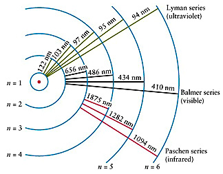
Some of the energy level transitions within the hydrogen atom have been given specific names. All transitions to/from the ground state (lowest energy level, n = 1) are part of the Lyman series. All transitions to/from the 1st excited stated (n = 2) are part of the Balmer series. All transitions to/from the 2nd excited state (n = 3) are part of the Paschen series. Other transitions also have formal names, but the Lyman, Balmer, and Paschen are the most commonly encountered.
Materials and Methods
Part A:
- Calculate E0, the ionization energy of hydrogen.
- Using the hydrogen lamp and the spectrometer with fiber optic cable, collect data for the emission spectrum of hydrogen.
- Fire up the hydrogen emission tube and clamp the end of the fiber optic up against it.
- Insert the cuvette end of the fiber into the spectrometer.
- Turn on the spectrometer. Its three LEDs will flash in succession.
- Start the Spectrometry software.
- Select “Analyze Light”
- Select the “Record” button (bottom left) to start acquiring data.
- Tweak the integration time and number of averages in order to obtain a large (but not cut off) signal. You may need to use different values of these parameters for different emission peaks. You should be able to locate 3 or possibly 4 emission peaks by judiciously adjusting the integration time and signal averaging.
- Use “Autoscale Display” and/or click and drag on the axes to zoom the plot.
- Use the “Coordinate Tool” to extract the wavelength of each peak. This tool is a box that snaps onto a peak when you drag it nearby. You may want to stop acquiring data while doing this (click the “Stop Record” button on lower left).
-
- Calculate the photon energy Ephoton (in eV) corresponding to each wavelength in the emission spectrum.
- Guess (or look up from a diagram of H emission spectra) ni for each wavelength. The spectrometer can only see H emission in the Balmer series (nf = 2). Calculate the quantity (1/nf2 – 1/ni2) for each photon.
- Plot Ephoton vs (1/nf2 – 1/ni2). From the equation for Ephoton above, you can see that you should obtain a straight line that goes through the origin; its slope is E0. When you do your fit, make sure you constrain the trend line so that it goes through the origin.
- Compare your value for E0 (from the plot) to the accepted value of 13.67 eV. How well do they agree? Calculate E0 using your data.
- Using the hydrogen lamp and the spectrometer with fiber optic cable, collect data for the emission spectrum of hydrogen.
Part B:
- Compare and contrast the normal solar light spectrum, the spectrum from an LED lamp, and the spectrum from an incandescent light.
- Hold the spectrometer’s fiber optic end up to a white LED lamp (for instance, the “flash” from your phone and to the incandescent lamp and record their spectra. You may want to use the lens to collect more light.
- Record the Sun’s spectrum. Hopefully you’ll be able to do this by standing near the window, but if necessary you can plug the spectrometer into your laptop and take it outside. You will need the software, which is available on the Using our spectrometer page.
- Compare two greens.
- In the spectrometer’s “Analyze Light” mode, measure the spectrum of the green LED on the top of the spectrometer.
- Switch to “Analyze Solution” mode and measure the absorption of a cuvette full of green food coloring.
- Explain chlorophyll fluorescence
- Measure the absorption of chlorophyll.
- Measure the fluorescence spectrum of chlorophyll with excitation at 405 and 500 nm.
Hints
- If you are having trouble holding the optical fiber steady in front of the hydrogen tube, clamp it in place.
- The spectrometer is not terribly sensitive. You can see easily in light levels that are too low for it to record via the fiber optic insert. Also, your vision adapts effortlessly to a huge range of light levels, so you are probably a very poor judge of whether a source is bright enough to be measured by the spectrometer.
- You can use a lens to capture more light. Hold the fiber optic cable at the focus of the lens.
- Be gentle with the fiber optic cable.
- Wifi connection
- The spectrometers do have a WiFi connection, but the WiFi on the lab computers is permanently disabled. You can connect with the USB cable, though.
- You may need to manually pair your spectrometer with your computer if you are using WiFi. Check the number on the bottom of the spectrometer to ensure you connect to the correct one!
- In Absorbance / Transmittance mode, you will need to first take “Dark” and “Blank” measurements. See the Using our spectrometer page on our website for guidance, look at the documentation from the manufacturer (PASCO), or ask a TA for help.
- All our samples are dissolved in ethanol (EthOH) so you should use plain EthOH as the blank.
Writeup
Use Lab 10 blank as a template for your lab writeup.
Questions to be answered
- Which series of emission lines is visible in the hydrogen emission spectrum?
- Calculate E0 (the constant in the Bohr formula for the hydrogen atom) and compare it to the accepted value of 13.6 eV.
- Which artificial light source (the LED or the incandescent light) is likely to reproduce the effect of natural light more closely? Though this is a qualitative question, answer with reference to the quantitative spectra you recorded.
- Compare and contrast (with measured spectra) the mechanism by which a green LED looks “green” and by which green food coloring looks “green”.
- Characterize and explain the similarities and differences between the emission spectra of chlorophyll with excitation at 500 nm and at 405 nm. In particular,
- Why is the 405 nm emission spectrum so much bigger than the 500 nm curve? You will want to refer to the absorption spectrum.
- You may see an extra bump in the 500 nm emission spectrum at around 500 nm (compared to the 405 nm emission spectrum). Where does this come from? Hint: it’s not real.
- In our experiment, chlorophyll in solution absorbs photons and then re-emits their energy as fluorescence photons, which is kind of pointless. Inside a cell, the energy absorbed by chlorophyll as passed along to an electron acceptor (eventually making a transmembrane potential that can be used to, for instance, make ATP from ADP). Assuming that the emitted photon energy (for chlorophyll in solution) is the same as the donor electron energy (for chlorophyll in a chloroplast), estimate the % efficiency for photosynthesis using 405 nm light.